This figure shows the absolute value of the wave function as a function of position. It is animated over time to illustrate the evolution of the state.
Figure 2: 3D Plot of Re(Ψ), Im(Ψ), x, Animated by Time
This figure provides a 3D visualization of the real and imaginary parts of the wave function. The animation shows how these components change over time.
Figure 3: 3D Plot of Eigenstates and Their Rotation as a Function of Time
This figure depicts the eigenstates of the Hamiltonian. It shows how these states rotate over time while maintaining their orthonormality.
Time Dependent Shrodinger Equation
iℏ∂t∂∣Ψ⟩=H^∣Ψ⟩
H^ is the hamiltonian
H^=−2mℏ2∇2+V^
Basis
we use the descrete orthonormal basis. the basis is formed by the eigenstates of the
position operator X^
Construction
split the interval [0,1] into N points
Δx=N−11
xi=i⋅Δx∀i∈{0,…,1}
dot product
⟨i∣j⟩=δij
Representation
∣i⟩ represents the point at xi
can be represented as the column vector
(0…1…0), where the 1 is at the ith position
any state Ψ(x) can be represented as ∑n=0N−1cn∣n⟩
where cn=Ψ(xn)
any operator O^ can be represented in the form of a matrix
Oij=⟨i∣O^∣j⟩
Eg: Identity I^
Iij=⟨i∣I^∣j⟩=⟨i∣j⟩=δij
this is the diagonal matrix with all diagonal entries 1
this also proves the completeness of our basis
Eg: Position X^
Xij=⟨i∣X^∣j⟩
as X^∣j⟩=xj∣j⟩
Xij=xj⟨i∣j⟩=xjδij
this is a diagonal matrix with the positions as diagonal entries
Harmonic Potential
what is a harmonic oscillator
why is studying it useful
V(x)=21mω2(x−21)2
V^=21mω2[X^−I^/2]2
Laplacian operator ∇2^
To approximate the laplacian in our basis, we can use the secant-line method
∂x2∂2≈Δx2xi+1+xi−1−2xi
∇2^≈∑nΔx2∣n+1⟩⟨n∣+∣n−1⟩⟨n∣−2∣n⟩⟨n∣
We can combine the potential and kinetic energy terms to get the hamiltonian H^
We can then use Euler’s method to evolve the state function
∣Ψ′⟩=(I^−ℏiΔtH^)∣Ψ⟩
But we can do better
as our hamiltonian is time independent, we can evaluate ∣Ψ(t)⟩ directly given ∣Ψ(0)⟩
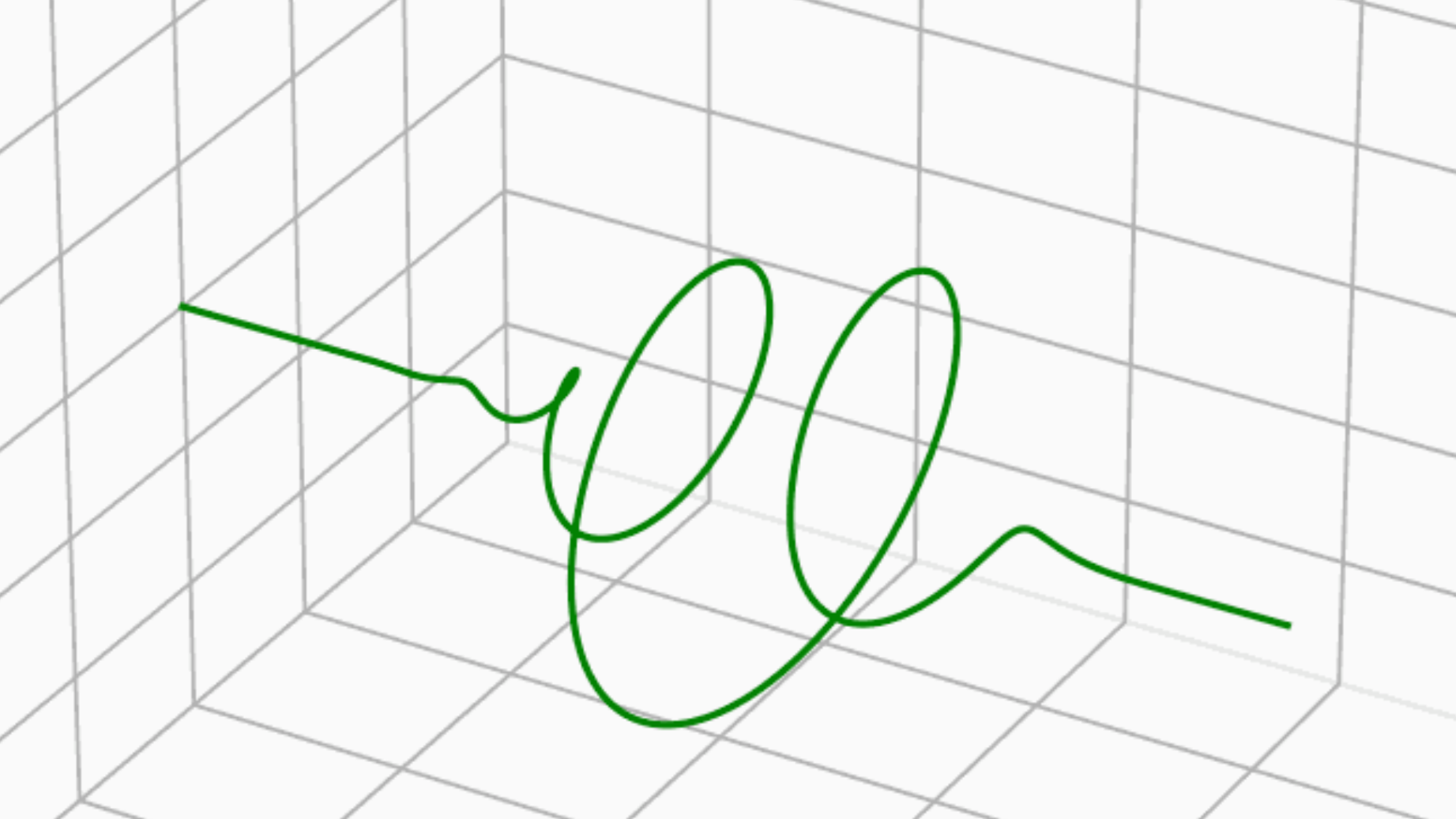
 This figure provides a 3D visualization of the real and imaginary parts of the wave function. The animation shows how these components change over time.
 This figure depicts the eigenstates of the Hamiltonian. It shows how these states rotate over time while maintaining their orthonormality.